Figure 7.5: State Diagram for the Mod-6 Counter.
| Contents | Previous Chapter | Next Chapter |
In a first practical application a modulo-6 counter will be developed. With this example the general development phases can be demonstrated.
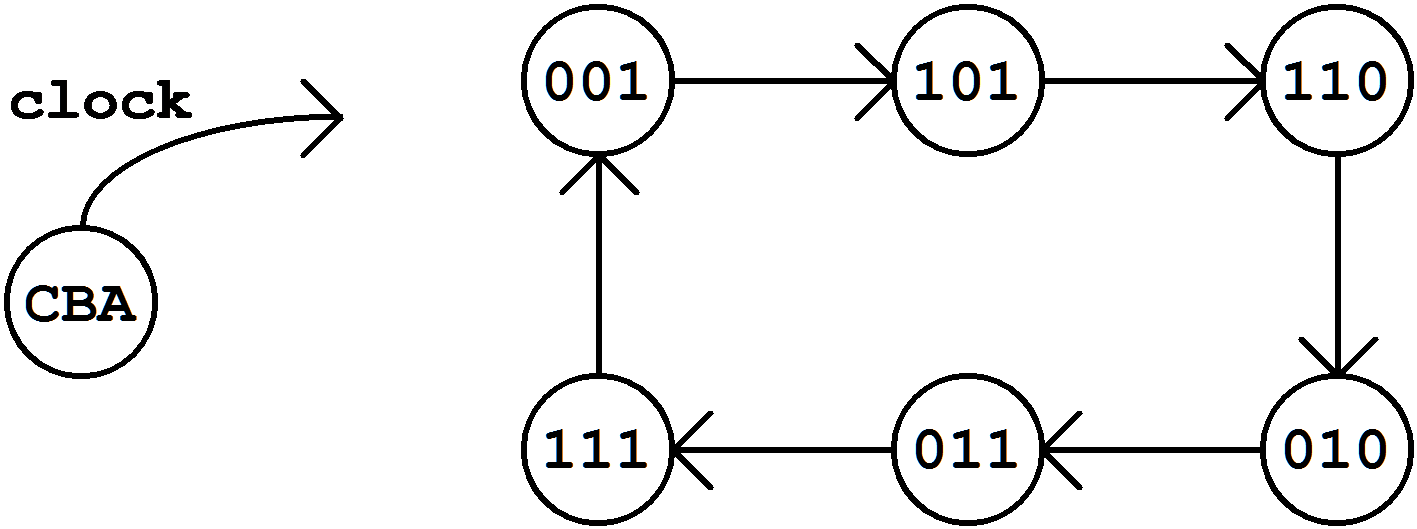
This counter is supposed to count in a sequence which is defined by the following state transition diagram:
Figure 7.5: State Diagram for the Mod-6 Counter.
In order to optimise the counting speed, this design should work without an output combinational circuit. Therefore the counting sequence will correspond to the state coding.
Hint:
In the above state coding (state diagram) the code '000' was intentionally omitted. In fact this state could easily be realized with a "reset" of the flip-flops. But in most cases this transition happens asynchronously and can therefore lead to system disturbances at the counter output.
Counters are developed in a form that can be called a "top-down" method: the process starts with a general description and ends with the circuit-oriented realization.
The following two development phases can therefore be distinguished:
Step 1:
Determination of the required number of Flip-Flops and the State Coding.
Considering a predefined counting range "modulo-m", then for a binary coding at least n flip-flops are required, with:
Besides this "effective" binary coding of the states there are other coding methods, which however almost always require a higher number of flip-flops (e.g. the "1-of-n" code or single-step codes like the Gray code or the Johnson counting code, see chapter 2 and 8). In the "1-of-n" code for instance one bit is assigned to each state, so that in this case exactly 2n flip-flops will be required.
In the design example (modulo-6 counter) only three flip-flops are required. Considering that therefore the total number of state codings is 2n = 8, two unused states will exist (free "triades" or "pseudo-triades") : '000' and
'100'.
Step 2:
Flip-Flop type selection and design of the combinational circuit.
The flip-flops mostly used are the D flip-flops or (because of the larger functional coverage) the JK flip-flops. The triggering is single-edged (controlled by the leading or trailing edge). In a synchronous counter all the flip-flop inputs must be defined for each state transition.
Starting with the state diagram the counting sequence will first be represented independently of the flip-flop type in a transition diagram (possibly using an optional transition table).
After this follows a FF specific representation in K-Maps, that in this connection are called application diagrams.
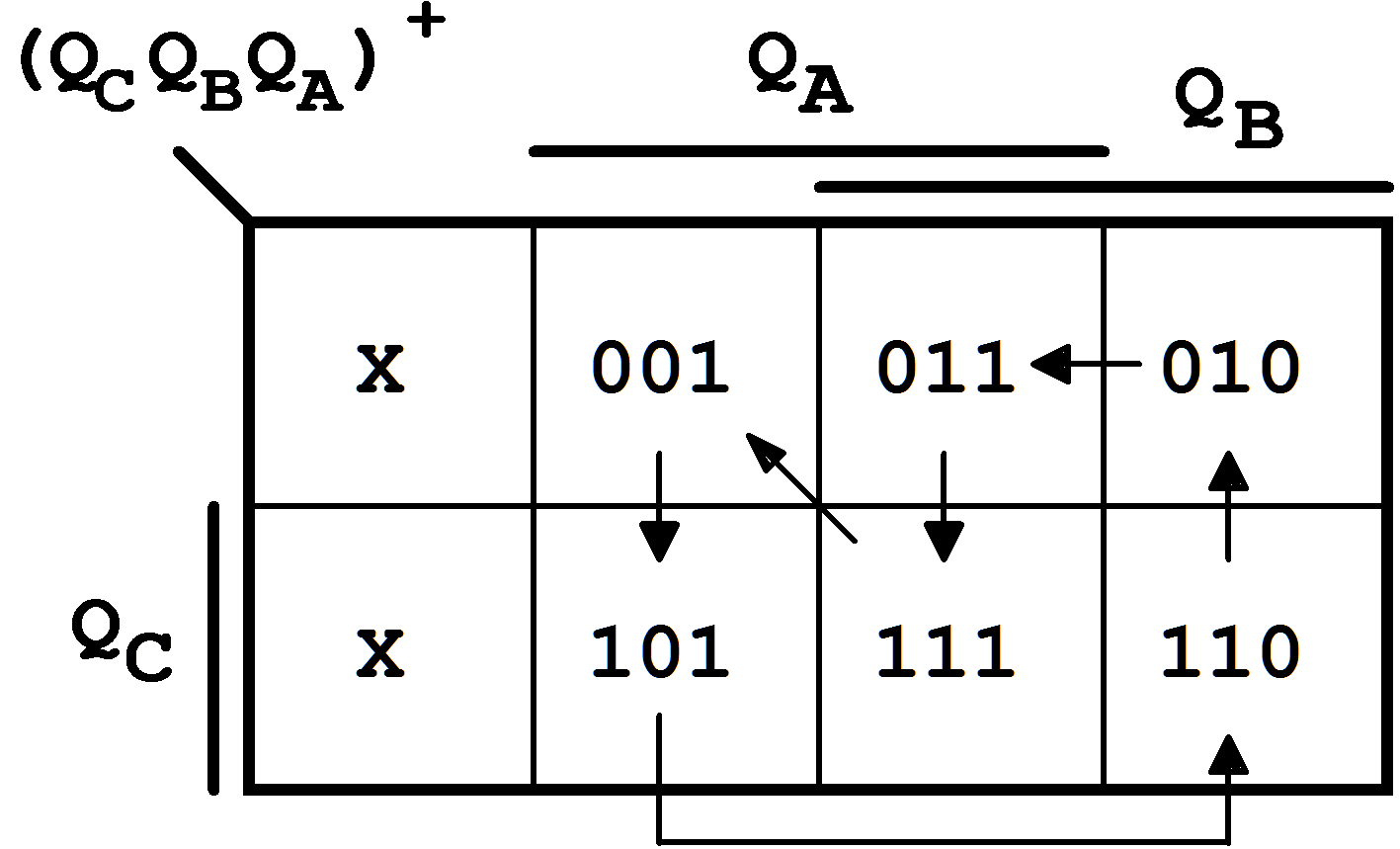
Figure 7.6: Transition map for the mod-6 counter.
In each field of this transition diagram the counter reading will be entered in the given coding (here
QCQBQA) . Thus the entry corresponds to the field coordinates. Then the counting sequence will be indicated using arrows, so that already in this arrangement the change of the individual bits becomes visible.
To find the solution with D flip-flops the necessary values for the inputs Di will be entered into individual K-Maps. This collection of diagrams is referred to as application diagrams.
For D flip-flops this is especially easy, because the following always applies:
| . | (7.1) |
For each state bit an application diagram is established, in which each field contains the value that the state bit will assume according to the transition diagram with the next clock signal:
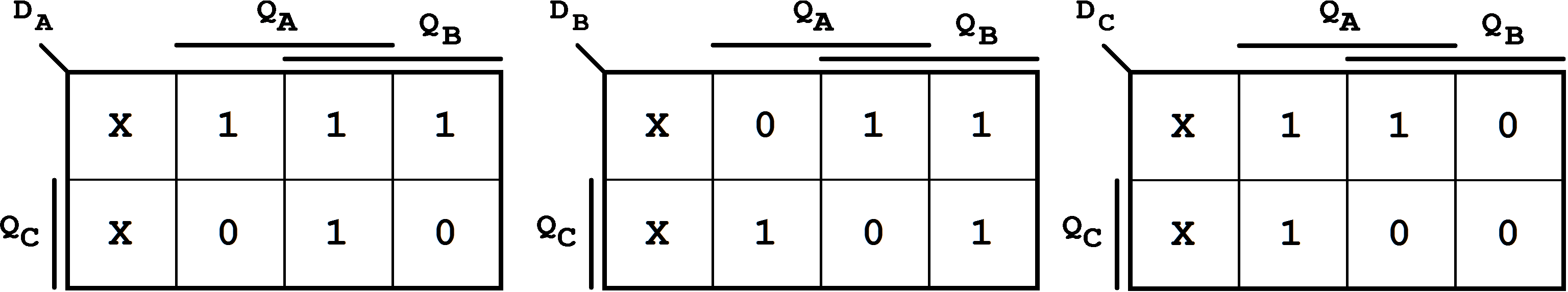
Figure 7.7: Application Diagrams for the Modulo-6 Counter.
From these application diagrams the Boolean functions for the inputs
Di can then be derived (after forming implicants):
 | (7.2) |
For a counter design using JK flip-flops it is advantageous to arrange the transition diagram directly in a JK specific way.
Therefore it makes sense to indicate the value changes of the state bits directly in the K-Map. Deriving the necessary control signals for the flip-flops can be immediately done with this specification Q → Q+.
From the transition diagram for a modulo-6 counter realization with D flip-flops (see above) the following transition diagrams for the equivalent construction with JK flip-flops can be defined:
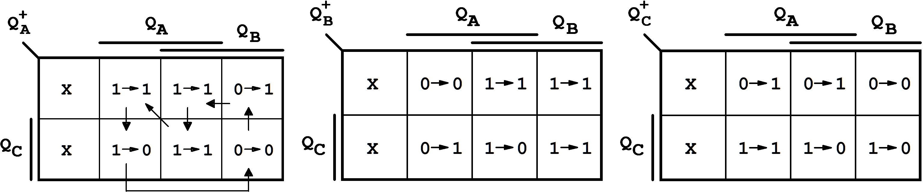
Figure 7.8: Transition Diagrams for the Modulo-6 Counter.
Figure 7.9: Transition Table for the JK Flip-flop.
Observing the already known transition table of the JK flip-flop the corresponding application diagrams can be derived from these transition diagrams.

Figure 7.10: Application Diagrams for the Modulo-6 Counter in JK Realization (with implicants formed for simplification).
From the K-Maps the functions for Ji and Ki can now be determined. For instance for flip-flop A the result is:
 | (7.3) |
The J-K control can also be developed using the characteristic function of the JK flip-flop:
| , |
and for QA, respectively:
| . |
From Fig. 7.8 follows:
| (7.5) |
Through comparison of Equ. 7.4 and Equ. 7.5 the solution given in Equ. 7.3 follows. Correspondingly the solutions for QB and QC can be determined.
| Contents | Previous Chapter | Next Chapter |